Linear Algebra

Linear Systems
Summary

Vector Spaces
Summary

Maps Between Spaces
Summary

Determinants
Summary

Similarity
Summary

Linear Systems

Solving Linear Systems
Summary

Linear Geometry of n-Space
Summary

Reduced Echelon Form
Summary

Topics about Linear Systems
Summary

Solving Linear Systems

Systems of linear equations are common in science and mathematics. These two examples from high school science (O'Nan 1990) give a sense of how they arise.

The first example is from Physics. Suppose that we are given three objects, one with a mass known to be 2 kg, and are asked to find the unknown masses. Suppose further that experimentation with a meter stick produces these two balances.

Since the sum of moments on the left of each balance equals the sum of moments on the right (the moment of an object is its mass times its distance from the balance point), the two balances give this system of two equations.

The second example of a linear system is from Chemistry. We can mix, under controlled conditions, toluene C₇H₈ and nitric acid HNO₃ to produce trinitrotoluene C₇H₅O₆N₃ along with the byproduct water (conditions have to be controlled very well, indeed— trinitrotoluene is better known as TNT). In what proportion should those components be mixed? The number of atoms of each element present before the reaction

must equal the number present afterward. Applying that principle to the elements C, H, N, and O in turn gives this system.

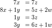
To finish each of these examples requires solving a system of equations. In each, the equations involve only the first power of the variables. This chapter shows how to solve any such system.

Gauss' Method
Summary

Describing the Solution Set
Summary

General = Particular + Homogenous
Summary

Comparing Set Descriptions
Summary

Automation
Summary

Topics about Linear Systems

Computer Algebra Systems
Summary

Input-Output Analysis
Summary

Accuracy of Computations
Summary

Analyzing Networks
Summary

Speed of Gauss' Method
Summary

Gauss' Method

Definition 1.1

A linear equation in variables x₁, x₂ , ... , x_n has the form

$a_1x_1+a_2x_2+a_3x_3+cdots+a_nx_n=d$

where the numbers a₁, a₂ , ... , a_n ∈ ℜ are the equation's coefficients and d ∈ ℜ is the constant. An n-tuple (s₁, s₂ , ... , s_n) ∈ ℜ is a solution of, or satisfies, that equation if substituting the numbers s₁, ... , s_n for the variables gives a true statement:

$a_1s_1+a_2s_2+ldots+a_ns_n=d$

.

A system of linear equations

$begin{array}{*{4}{rc}r} a_{1,1}x_1 &+ &a_{1,2}x_2 &+ &cdots &+ &a_{1,n}x_n &= &d_1 a_{2,1}x_1 &+ &a_{2,2}x_2 &+ &cdots &+ &a_{2,n}x_n &= &d_2 & & & & & & &vdots a_{m,1}x_1 &+ &a_{m,2}x_2 &+ &cdots &+ &a_{m,n}x_n &= &d_m end{array}$

has the solution (s₁, s₂ , ... , s_n) if that n-tuple is a solution of all of the equations in the system.

Example 1.2

The ordered pair (-1 , 5) is a solution of this system

$begin{array}{*{2}{rc}r} 3x_1 &+ &2x_2 &= &7 -x_1 &+ &x_2 &= &6 end{array}$

In contrast, (5 , -1) is not a solution.

Finding the set of all solutions is solving the system. No guesswork or good fortune is needed to solve a linear system. There is an algorithm that always works. The next example introduces that algorithm, called Gauss' method. It transforms the system, step by step, into one with a form that is easily solved.

Example 1.3

To solve this system

$begin{array}{*{3}{rc}r} & & & &3x_3 &= &9 x_1 &+ &5x_2 &- &2x_3 &= &2 frac{1}{3}x_1 &+ &2x_2 & & &= &3 end{array}$

we repeatedly transform it until it is in a form that is easy to solve.

$begin{array}{rcl} quad &xrightarrow[]{ text{swap row 1 with row 3} } &begin{array}{*{3}{rc}r} frac{1}{3}x_1 &+ &2x_2 & & &= &3 x_1 &+ &5x_2 &- &2x_3 &= &2 & & & &3x_3 &= &9 end{array} &xrightarrow[]{ text{multiply row 1 by 3} } &begin{array}{*{3}{rc}r} x_1 &+ &6x_2 & & &= &9 x_1 &+ &5x_2 &- &2x_3 &= &2 & & & &3x_3 &= &9 end{array} &xrightarrow[]{ text{add }-1text{ times row 1 to row 2} } &begin{array}{*{3}{rc}r} x_1 &+ &6x_2 & & &= &9 & &-x_2 &- &2x_3 &= &-7 & & & &3x_3 &= &9 end{array} end{array}$

The third step is the only nontrivial one. We've mentally multiplied both sides of the first row by -1, mentally added that to the old second row, and written the result in as the new second row.

Now we can find the value of each variable. The bottom equation shows that x₃ = 3. Substituting 3 for x₃ in the middle equation shows that x₂ = 1. Substituting those two into the top equation gives that x₁ = 3 and so the system has a unique solution: the solution set is { ( 3 , 1 , 3 ) }.

Most of this subsection and the next one consists of examples of solving linear systems by Gauss' method. We will use it throughout this book. It is fast and easy. But, before we get to those examples, we will first show that this method is also safe in that it never loses solutions or picks up extraneous solutions.

Theorem 1.4 (Gauss' method)

If a linear system is changed to another by one of these operations

an equation is swapped with another
an equation has both sides multiplied by a nonzero constant
an equation is replaced by the sum of itself and a multiple of another

then the two systems have the same set of solutions.

Each of those three operations has a restriction. Multiplying a row by 0 is not allowed because obviously that can change the solution set of the system. Similarly, adding a multiple of a row to itself is not allowed because adding -1 times the row to itself has the effect of multiplying the row by 0. Finally, swapping a row with itself is disallowed to make some results in the fourth chapter easier to state and remember (and besides, self-swapping doesn't accomplish anything).

Title
Summary