Solving Linear Systems

Systems of linear equations are common in science and mathematics. These two examples from high school science (O'Nan 1990) give a sense of how they arise.

The first example is from Physics. Suppose that we are given three objects, one with a mass known to be 2 kg, and are asked to find the unknown masses. Suppose further that experimentation with a meter stick produces these two balances.

Since the sum of moments on the left of each balance equals the sum of moments on the right (the moment of an object is its mass times its distance from the balance point), the two balances give this system of two equations.

The second example of a linear system is from Chemistry. We can mix, under controlled conditions, toluene C₇H₈ and nitric acid HNO₃ to produce trinitrotoluene C₇H₅O₆N₃ along with the byproduct water (conditions have to be controlled very well, indeed— trinitrotoluene is better known as TNT). In what proportion should those components be mixed? The number of atoms of each element present before the reaction

must equal the number present afterward. Applying that principle to the elements C, H, N, and O in turn gives this system.

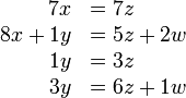
To finish each of these examples requires solving a system of equations. In each, the equations involve only the first power of the variables. This chapter shows how to solve any such system.

Gauss' Method
If a linear system is changed to another by one of these operations
     1. an equation is swapped with another
    2. an equation has both sides multiplied by a nonzero constant
    3. an equation is replaced by the sum of itself and a multiple of another
 then the two systems have the same set of solutions.

Gauss' method uses these three row operations to set a system up for back substitution. If any step shows a contradictory equation then we can stop with the conclusion that the system has no solutions. If we reach echelon form without a contradictory equation, and each variable is a leading variable in its row, then the system has a unique solution and we find it by back substitution. Finally, if we reach echelon form without a contradictory equation, and there is not a unique solution (at least one variable is not a leading variable) then the system has many solutions.

Describing the Solution Set
Summary

General = Particular + Homogenous
Summary

Comparing Set Descriptions
Summary

Automation
Summary

Linear Geometry of n-Space

In the first section, we had to do a bit of work to show that there are only three types of solution sets— singleton, empty, and infinite. But in the special case of systems with two equations and two unknowns this is easy to see. Draw each two-unknowns equation as a line in the plane and then the two lines could have a unique intersection, be parallel, or be the same line.

Unique solution

3x + 2y = 7
x - y = -1

No solutions

3x + 2y = 7
3x + 2y = 4

Infinitely many solutions

3x + 2y = 7
6x + 4y = 14

These pictures don't prove the results from the prior section, which apply to any number of linear equations and any number of unknowns, but nonetheless they do help us to understand those results. This section develops the ideas that we need to express our results from the prior section, and from some future sections, geometrically. In particular, while the two-dimensional case is familiar, to extend to systems with more than two unknowns we shall need some higher-dimensional geometry.

Vectors in Space
Summary

Length and Angle Measures
Summary

Reduced Echelon Form

After developing the mechanics of Gauss' method, we observed that it can be done in more than one way. One example is that we sometimes have to swap rows and there can be more than one row to choose from. Another example is that from this matrix

Gauss' method could derive any of these echelon form matrices.

The first results from -2ρ₁ + ρ₂. The second comes from following (1/2)ρ₁ with -4ρ_{1 +} ρ₂. The third comes from -2ρ_{1 +} ρ₂ followed by 2ρ_{2 +} ρ₁ (after the first pivot the matrix is already in echelon form so the second one is extra work but it is nonetheless a legal row operation).

The fact that the echelon form outcome of Gauss' method is not unique leaves us with some questions. Will any two echelon form versions of a system have the same number of free variables? Will they in fact have exactly the same variables free? In this section we will answer both questions "yes". We will do more than answer the questions. We will give a way to decide if one linear system can be derived from another by row operations. The answers to the two questions will follow from this larger result.

Gauss-Jordan Reduction
Summary

Row Equivalence
Summary

Topics about Linear Systems

Computer Algebra Systems
Summary

Input-Output Analysis
Summary

Accuracy of Computations
Summary

Analyzing Networks
Summary

Speed of Gauss' Method
Summary

Definition of Vector Spaces

We shall study structures with two operations, an addition and a scalar multiplication, that are subject to some simple conditions. We will reflect more on the conditions later, but on first reading notice how reasonable they are. For instance, surely any operation that can be called an addition (e.g., column vector addition, row vector addition, or real number addition) will satisfy all the conditions in Definition 1.1 below.

Definition and Examples
Summary

Subspaces and Spanning sets
Summary

Linear Independence

The prior section shows that a vector space can be understood as an unrestricted linear combination of some of its elements— that is, as a span. For example, the space of linear polynomials \( {a+bx|a,b}∈\mathbb{R} \) { a + bx | a , b } ∈ ℜ is spanned by the set { 1 , x }. The prior section also showed that a space can have many sets that span it. The space of linear polynomials is also spanned by { 1 , 2x } and { 1 , x , 2x } .

At the end of that section we described some spanning sets as "minimal", but we never precisely defined that word. We could take "minimal" to mean one of two things. We could mean that a spanning set is minimal if it contains the smallest number of members of any set with the same span. With this meaning { 1 , x , 2x } is not minimal because it has one member more than the other two. Or we could mean that a spanning set is minimal when it has no elements that can be removed without changing the span. Under this meaning { 1 , x , 2x } is not minimal because removing the 2x and getting { 1 , x } leaves the span unchanged.

The first sense of minimality appears to be a global requirement, in that to check if a spanning set is minimal we seemingly must look at all the spanning sets of a subspace and find one with the least number of elements. The second sense of minimality is local in that we need to look only at the set under discussion and consider the span with and without various elements. For instance, using the second sense, we could compare the span of { 1 , x , 2x } with the span of { 1 , x }   and note that the 2x is a "repeat" in that its removal doesn't shrink the span.

In this section we will use the second sense of "minimal spanning set" because of this technical convenience. However, the most important result of this book is that the two senses coincide; we will prove that in the section after this one.

Definition and Examples
Summary

Basis and Dimensions

The prior section ends with the statement that a spanning set is minimal when it is linearly independent and a linearly independent set is maximal when it spans the space. So the notions of minimal spanning set and maximal independent set coincide. In this section we will name this idea and study its properties.

Basis
Summary

Dimension
Summary

Vector Spaces and Linear Systems
Summary

Combining Subspaces
Summary

Topics about Vector Spaces

Fields
Summary

Crystals
Summary

Voting Paradoxes
Summary

Dimensional Analysis
Summary

Isomorphisms

In the examples following the definition of a vector space we developed the intuition that some spaces are "the same" as others. For instance, the space of two-tall column vectors and the space of two-wide row vectors are not equal because their elements—column vectors and row vectors—are not equal, but we have the idea that these spaces differ only in how their elements appear. We will now make this idea precise.

This section illustrates a common aspect of a mathematical investigation. With the help of some examples, we've gotten an idea. We will next give a formal definition, and then we will produce some results backing our contention that the definition captures the idea. We've seen this happen already, for instance, in the first section of the Vector Space chapter. There, the study of linear systems led us to consider collections closed under linear combinations. We defined such a collection as a vector space, and we followed it with some supporting results.

Of course, that definition wasn't an end point, instead it led to new insights such as the idea of a basis. Here too, after producing a definition, and supporting it, we will get two surprises (pleasant ones). First, we will find that the definition applies to some unforeseen, and interesting, cases. Second, the study of the definition will lead to new ideas. In this way, our investigation will build a momentum.

Definition and Examples
Summary

Dimension Characterizes Isomorphism
Summary

Homomorphisms

The definition of isomorphism has two conditions. In this section we will consider the second one, that the map must preserve the algebraic structure of the space. We will focus on this condition by studying maps that are required only to preserve structure; that is, maps that are not required to be correspondences.

Experience shows that this kind of map is tremendously useful in the study of vector spaces. For one thing, as we shall see in the second subsection below, while isomorphisms describe how spaces are the same, these maps describe how spaces can be thought of as alike.

Definition of Homomorphism
Summary

Rangespace and Nullspace
Summary

Computing Linear Maps

The prior section shows that a linear map is determined by its action on a basis. In fact, the equation

shows that, if we know the value of the map on the vectors in a basis, then we can compute the value of the map on any vector

at all. We just need to find the

c

's to express

with respect to the basis.

This section gives the scheme that computes, from the representation of a vector in the domain

, the representation of that vector's image in the codomain

, using the representations of

, ...,

.

Representing Linear Maps with Matrices
Summary

Any Matrix Represents a Linear Map
Summary

Matrix Operations

The prior section shows how matrices represent linear maps. A good strategy, on seeing a new idea, is to explore how it interacts with some already-established ideas. In the first subsection we will ask how the representation of the sum of two maps f + g is related to the representations of the two maps, and how the representation of a scalar product r · h of a map is related to the representation of that map. In later subsections we will see how to represent map composition and map inverse.

Sums and Scalar Products
Summary

Matrix Multiplication
Summary

Mechanics of Matrix Multiplication
Summary

Inverses
Summary

Change of Basis

Representations, whether of vectors or of maps, vary with the bases. For instance, with respect to the two bases

and

for

, the vector

has two different representations.

Similarly, with respect to

and

, the identity map has two different representations.

With our point of view that the objects of our studies are vectors and maps, in fixing bases we are adopting a scheme of tags or names for these objects, that are convienent for computation. We will now see how to translate among these names— we will see exactly how representations vary as the bases vary.

Changing Representations of Vectors
Summary

Changing Map Representations
Summary

Projections

We have described the projection

from

into its

plane subspace as a "shadow map". This shows why, but it also shows that some shadows fall upward.

So perhaps a better description is: the projection of

is the

in the plane with the property that someone standing on

and looking straight up or down sees

. In this section we will generalize this to other projections, both orthogonal (i.e., "straight up and down") and nonorthogonal.

Orthogonal Projection Onto a Line
Summary

Gram-Schmidt Orthogonalization
Summary

Projection Onto a Subspace
Summary

Topics about Maps Between Spaces

Line of Best Fit
Summary

Geometry of Linear Maps
Summary

Markov Chains
Summary

Orthonormal Matrices
Summary

Definition

For 1 × 1 matrices, determining nonsingularity is trivial.

is nonsingular iff

The 2 × 2 formula came out in the course of developing the inverse.

is nonsingular iff

The 3 × 3 formula can be produced similarly (see Problem 9).

is nonsingular iff

With these cases in mind, we posit a family of formulas,

,

, etc.

For each

the formula gives rise to a determinant function

such that an

matrix

is nonsingular if and only if

. (We usually omit the subscript because if

is

then "

" could only mean "

".)

Exploration
Summary

Properties of Determinants
Summary

The Permutation Expansion
Summary

Determinants Exist
Summary

Geometry of Determinants

The prior section develops the determinant algebraically, by considering what formulas satisfy certain properties. This section complements that with a geometric approach. One advantage of this approach is that, while we have so far only considered whether or not a determinant is zero, here we shall give a meaning to the value of that determinant. (The prior section handles determinants as functions of the rows, but in this section columns are more convenient. The final result of the prior section says that we can make the switch.)

Determinants as Size Functions
Summary

Other Formulas for Determinants

Determinants are a fount of interesting and amusing formulas. Here is one that is often seen in calculus classes and used to compute determinants by hand.

Laplace's Expansion
Summary

Topics about Determinants

Cramer's Rule
Summary

Speed of Calculating Determinants
Summary

Projective Geometry
Summary

Complex Vector Spaces

This chapter requires that we factor polynomials. Of course, many polynomials do not factor over the real numbers; for instance, x² + 1 does not factor into the product of two linear polynomials with real coefficients. For that reason, we shall from now on take our scalars from the complex numbers.

That is, we are shifting from studying vector spaces over the real numbers to vector spaces over the complex numbers— in this chapter vector and matrix entries are complex.

Any real number is a complex number and a glance through this chapter shows that most of the examples use only real numbers. Nonetheless, the critical theorems require that the scalars be complex numbers, so the first section below is a quick review of complex numbers.

In this book we are moving to the more general context of taking scalars to be complex only for the pragmatic reason that we must do so in order to develop the representation. We will not go into using other sets of scalars in more detail because it could distract from our goal. However, the idea of taking scalars from a structure other than the real numbers is an interesting one. Delightful presentations taking this approach are in (Halmos 1958) and (Hoffman & Kunze 1971).

Factoring and Complex Numbers: A Review
Summary

Complex Representations
Summary

Similarity

Definition and Examples
Summary

Diagonalizability
Summary

Eigenvalues and Eigenvectors
Summary

Nilpotence

The goal of this chapter is to show that every square matrix is similar to one that is a sum of two kinds of simple matrices. The prior section focused on the first kind, diagonal matrices. We now consider the other kind.

Self-Composition
Summary

Strings
Summary

Jordan Form

This section uses material from three optional subsections: Direct Sum, Determinants Exist, and Other Formulas for the Determinant.

The chapter on linear maps shows that every

can be represented by a partial-identity matrix with respect to some bases

and

. This chapter revisits this issue in the special case that the map is a linear transformation

. Of course, the general result still applies but with the codomain and domain equal we naturally ask about having the two bases also be equal. That is, we want a canonical form to represent transformations as

.

After a brief review section, we began by noting that a block partial identity form matrix is not always obtainable in this

case. We therefore considered the natural generalization, diagonal matrices, and showed that if its eigenvalues are distinct then a map or matrix can be diagonalized. But we also gave an example of a matrix that cannot be diagonalized and in the section prior to this one we developed that example. We showed that a linear map is nilpotent— if we take higher and higher powers of the map or matrix then we eventually get the zero map or matrix— if and only if there is a basis on which it acts via disjoint strings. That led to a canonical form for nilpotent matrices.

Now, this section concludes the chapter. We will show that the two cases we've studied are exhaustive in that for any linear transformation there is a basis such that the matrix representation

is the sum of a diagonal matrix and a nilpotent matrix in its canonical form.

Polynomials of Maps and Matrices
Summary

Jordan Canonical Form
Summary

Topics about Similarity

Geometry of Eigenvalues
Summary

The Method of Powers
Summary

Stable Populations
Summary

Linear Recurrences
Summary