Gauss' Method

Definition 1.1

A linear equation in variables x₁ , x₂ , ... , x_n has the form

where the numbers a₁ , a₂ , ... , a_n ∈ ℜ are the equation's coefficients and d ∈ ℜ is the constant. An n-tuple (s₁ , s₂ , ... , s_n) ∈ ℜ is a solution of, or satisfies, that equation if substituting the numbers s₁ , ... , s_n for the variables gives a true statement:

A system of linear equations

has the solution (s₁ , s₂ , ... , s_n) if that n-tuple is a solution of all of the equations in the system.

Example 1.2

The ordered pair (-1 , 5) is a solution of this system

In contrast, (5 , -1) is not a solution.

Finding the set of all solutions is solving the system. No guesswork or good fortune is needed to solve a linear system. There is an algorithm that always works. The next example introduces that algorithm, called Gauss' method. It transforms the system, step by step, into one with a form that is easily solved.

Example 1.3

To solve this system

we repeatedly transform it until it is in a form that is easy to solve.

The third step is the only nontrivial one. We've mentally multiplied both sides of the first row by -1, mentally added that to the old second row, and written the result in as the new second row.

Now we can find the value of each variable. The bottom equation shows that x₃ = 3. Substituting 3 for x₃ in the middle equation shows that x₂ = 1. Substituting those two into the top equation gives that x₁ = 3 and so the system has a unique solution: the solution set is { ( 3 , 1 , 3 ) }.

Most of this subsection and the next one consists of examples of solving linear systems by Gauss' method. We will use it throughout this book. It is fast and easy. But, before we get to those examples, we will first show that this method is also safe in that it never loses solutions or picks up extraneous solutions.

Theorem 1.4 (Gauss' method)

If a linear system is changed to another by one of these operations

1. an equation is swapped with another
2. an equation has both sides multiplied by a nonzero constant
3. an equation is replaced by the sum of itself and a multiple of another

then the two systems have the same set of solutions.

Each of those three operations has a restriction. Multiplying a row by 0 is not allowed because obviously that can change the solution set of the system. Similarly, adding a multiple of a row to itself is not allowed because adding -1 times the row to itself has the effect of multiplying the row by 0. Finally, swapping a row with itself is disallowed to make some results in the fourth chapter easier to state and remember (and besides, self-swapping doesn't accomplish anything).

Proof

We will cover the equation swap operation here and save the other two cases for Problem 14.

Consider this swap of row i with row j

The n-tuple (s₁, s₂, ... , s_n) satisfies the system before the swap if and only if substituting the values, the s's, for the variables, the x's, gives true statements:

and ...

and ...

and ...

This is exactly the requirement that (s₁ , s₂ , ... , s_n) solves the system after the row swap.

Definition 1.5

The three operations from Theorem 1.4 are the elementary reduction operations, or row operations, or Gaussian operations. They are swapping, multiplying by a scalar or rescaling, and pivoting.

When writing out the calculations, we will abbreviate "row i" by "ρ_i". For instance, we will denote a pivot operation by kρ_i + ρ_j, with the row that is changed written second. We will also, to save writing, often list pivot steps together when they use the same ρ_i.

Example 1.6

A typical use of Gauss' method is to solve this system.

The first transformation of the system involves using the first row to eliminate the x in the second row and the x in the third. To get rid of the second row's 2x, we multiply the entire first row by -2, add that to the second row, and write the result in as the new second row. To get rid of the third row's x, we multiply the first row by -1, add that to the third row, and write the result in as the new third row

(Note that the two ρ₁ steps -2ρ₁ + ρ₂ and -ρ₁ + ρ₃ are written as one operation.) In this second system, the last two equations involve only two unknowns. To finish we transform the second system into a third system, where the last equation involves only one unknown. This transformation uses the second row to eliminate y from the third row.

Now we are set up for the solution. The third row shows that z = 0. Substitute that back into the second row to get y = -1, and then substitute back into the first row to get x = 1.

Example 1.7

For the Physics problem from the start of this chapter, Gauss' method gives this.

So c = 4, and back-substitution gives that h = 1. (The Chemistry problem is solved later.)

Example 1.8

The reduction

shows that z = 3 , y = -1 , and x = 7.

As these examples illustrate, Gauss' method uses the elementary reduction operations to set up back-substitution.

Definition 1.9

In each row, the first variable with a nonzero coefficient is the row's leading variable. A system is in echelon form if each leading variable is to the right of the leading variable in the row above it (except for the leading variable in the first row).

Example 1.10

The only operation needed in the examples above is pivoting. Here is a linear system that requires the operation of swapping equations. After the first pivot

the second equation has no leading y. To get one, we look lower down in the system for a row that has a leading y and swap it in.

(Had there been more than one row below the second with a leading y then we could have swapped in any one.) The rest of Gauss' method goes as before.

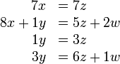
Back-substitution gives w = 1 , z = 2 , y = -1 , and x = -1 .

Strictly speaking, the operation of rescaling rows is not needed to solve linear systems. We have included it because we will use it later in this chapter as part of a variation on Gauss' method, the Gauss-Jordan method.

All of the systems seen so far have the same number of equations as unknowns. All of them have a solution, and for all of them there is only one solution. We finish this subsection by seeing for contrast some other things that can happen.

Example 1.11

Linear systems need not have the same number of equations as unknowns. This system

has more equations than variables. Gauss' method helps us understand this system also, since this

shows that one of the equations is redundant. Echelon form

gives y = 1 and x = -2 . The "0 = 0" is derived from the redundancy.

That example's system has more equations than variables. Gauss' method is also useful on systems with more variables than equations. Many examples are in the next subsection.

Another way that linear systems can differ from the examples shown earlier is that some linear systems do not have a unique solution. This can happen in two ways.

The first is that it can fail to have any solution at all.

Example 1.12

Contrast the system in the last example with this one.

Here the system is inconsistent: no pair of numbers satisfies all of the equations simultaneously. Echelon form makes this inconsistency obvious.

The solution set is empty.

Example 1.13

The prior system has more equations than unknowns, but that is not what causes the inconsistency— Example 1.11 has more equations than unknowns and yet is consistent. Nor is having more equations than unknowns sufficient for inconsistency, as is illustrated by this inconsistent system with the same number of equations as unknowns.

The other way that a linear system can fail to have a unique solution is to have many solutions.

Example 1.14

In this system

any pair of numbers satisfying the first equation automatically satisfies the second. The solution set {(x,y)| x + y = 4 } is infinite; some of its members are (0 , 4) , (-1 , 5) , and (2.5 , 1.5). The result of applying Gauss' method here contrasts with the prior example because we do not get a contradictory equation.

Don't be fooled by the "0 = 0" equation in that example. It is not the signal that a system has many solutions.

Example 1.15

The absence of a "0 = 0" does not keep a system from having many different solutions. This system is in echelon form

has no "0 = 0", and yet has infinitely many solutions. (For instance, each of these is a solution: (0 , 1, -1) , (0 , 1/2 , -1/2 ) ,  (0 , 0 , 0) , and (0 , -π , π) . There are infinitely many solutions because any triple whose first component is 0 and whose second component is the negative of the third is a solution.)

Nor does the presence of a "0 = 0" mean that the system must have many solutions. Example 1.11 shows that. So does this system, which does not have many solutions— in fact it has none— despite that when it is brought to echelon form it has a "0 = 0" row.

We will finish this subsection with a summary of what we've seen so far about Gauss' method.

Gauss' method uses the three row operations to set a system up for back substitution. If any step shows a contradictory equation then we can stop with the conclusion that the system has no solutions. If we reach echelon form without a contradictory equation, and each variable is a leading variable in its row, then the system has a unique solution and we find it by back substitution. Finally, if we reach echelon form without a contradictory equation, and there is not a unique solution (at least one variable is not a leading variable) then the system has many solutions.

The next subsection deals with the third case— we will see how to describe the solution set of a system with many solutions.

Exercises
Summary